Karpathy Bigram explained in 10min..

Back in 2023, Andre Karpathy released a video explaining how GPT works by building it from scratch. And in the first half of the video, he explained what's called Bagram language model before he even gets to GPT. And since this 2-hour video gets quite technical, I thought I can condense it down and explain it in two parts. And this video will cover the biogram portion. So let's start with a simple scenario. Let's say someone hands you a random model and asks you to train the model to sound like Shakespeare. How exactly do we do this? Of course, we need to start by gathering Shakespeare's archives first and then train the model with it. But what does it even mean to train the model with Shakespeare's data? Maybe what we can start with is looking at the entire Shakespeare's data and pulling out unique characters from the data set. We have alphabets like A to Z, some numbers, and special characters. And we find that there are 65 unique characters. Let's call them tokens that Shakespeare used in this entire data set. Perfect. This is a great place to start. Now that we have this entire vocabulary identified as a set, what we need to do is to try to make the model predict one token at a time and hopefully in the end it'll end up sounding like Shakespeare somehow. For example, if I start the sentence with a token T, I want the model now to finish the sentence by predicting one token at a time. And since there are 65 different possible tokens to choose from our vocabulary, all we have to do is to ask the model to predict the next token that comes after the token T and continue generating them until the sentence is finished. And of course, the added challenge here is to predict it like Shakespeare actually would. Now, if we expand this beyond just our token T to now represent all 65 tokens, it'll look something like this table where each row like the token T from earlier is just one row out of all 65 rows that represent every token used in the data. And all columns here also represent our entire vocabulary, which tells us given our current token, what the next likelihood token might be. And this table here is randomized since we didn't start training yet. So if we really wanted to know given our current randomized set what comes after the token T, it will choose the token semicolon as the next token. In fact, if we were to use this randomized table for inference without training, it will generate this randomized output that just sounds like gibberish. And we could continue generating different variations of this randomized table, hoping that it will somehow sound like Shakespeare at the end. But that's like trying to draw the Mona Lisa by randomly generating every pixel on the screen. Good luck with that. So our task is now clear. We need to push and pull these numerical representations in order to converge them toward what resembles more like what Shakespeare's data set looks like. Which means our goal here is to minimize the error that's already contained in the randomized table from high error state to low air state. Okay. Now, let's actually move on to training this model. But first, a quick word from Blue. Impact sponsoring this video. As we are undergoing this massive technological shift, I'm sure everywhere you go, you're hearing about AI as it relates to jobs, coding, disruptions here and disruptions there. And honestly, what's so uncertain is the pace of innovation in how fast AI will move as we saw in Enthropic's Mythos model. And the future of AI is really hard to grasp and only few frontier labs really hold the key to how the industry will unfold as a technology moves forward. So if you're curious about the bigger picture on how AI might impact humanity, Blue Dot is built to help people learn and contribute to the future of AI. Blue Dot Impact is a nonprofit company that draws people who are curious about AI to stay informed as we think about how AI might jive with humanity as a whole. The courses are completely free and funded philanthropically and the mission is to help people get involved. I find that it helps broaden my perspective beyond my own world, but think about the big picture as AI continues to improve. Link in the description below if you're interested. When we look at training this model with our given data set, we find that Shakespeare's data set contains a total of 1,75,394 characters in total. That's a lot. And technically we could try to run them all at once since this is a relatively small model. In reality that's not a very scalable approach for many reasons. In practice we divide this in chunks so we can train multiple chunks in parallel and under each chunk we set a block size which is a total number of tokens that are contained in each batch. So in other words, we take the small segment of the training data, split them into four batches and each batch might contain eight blocks of tokens where each token have its own row from the embedding table which has 65 dimensions like we saw earlier. To put it more clearly, let's say the sentence was the following quote to be or not to be. That is the we can split this into four chunks. And the first batch has eight characters to be or. And within this very batch, each token, there are 65 channels that help the model predict what comes after its current token. So given our current selection of four batches, eight blocks, and 65 channels, we have to figure out a way to change the model's embedding table to better represent Shakespeare's style. Let's say the token T in this example is followed by the token O, but in a different batch, it's also followed by the token H. As you can see, this means that we can't just simply penalize the rest of the tokens to all be zero and make the token O be the next token deterministically since it will set the value O to be zero again when the model processes the token H, which would make H the only possible token after the letter T. And beyond this specific example, there will be many different permutations of words that contain the token T to account for. So clearly we need a more sophisticated system in place than to actually zero everything out to properly update this table slowly as it converges towards Shakespearean embedding table. The first thing we need to do is measure the loss function. Meaning given our current batch, we need to find out how wrong are we given our current representation of the embedding table from Shakespeare. One of the most popular ways to measure this is by using what's called negative loss likelihood. 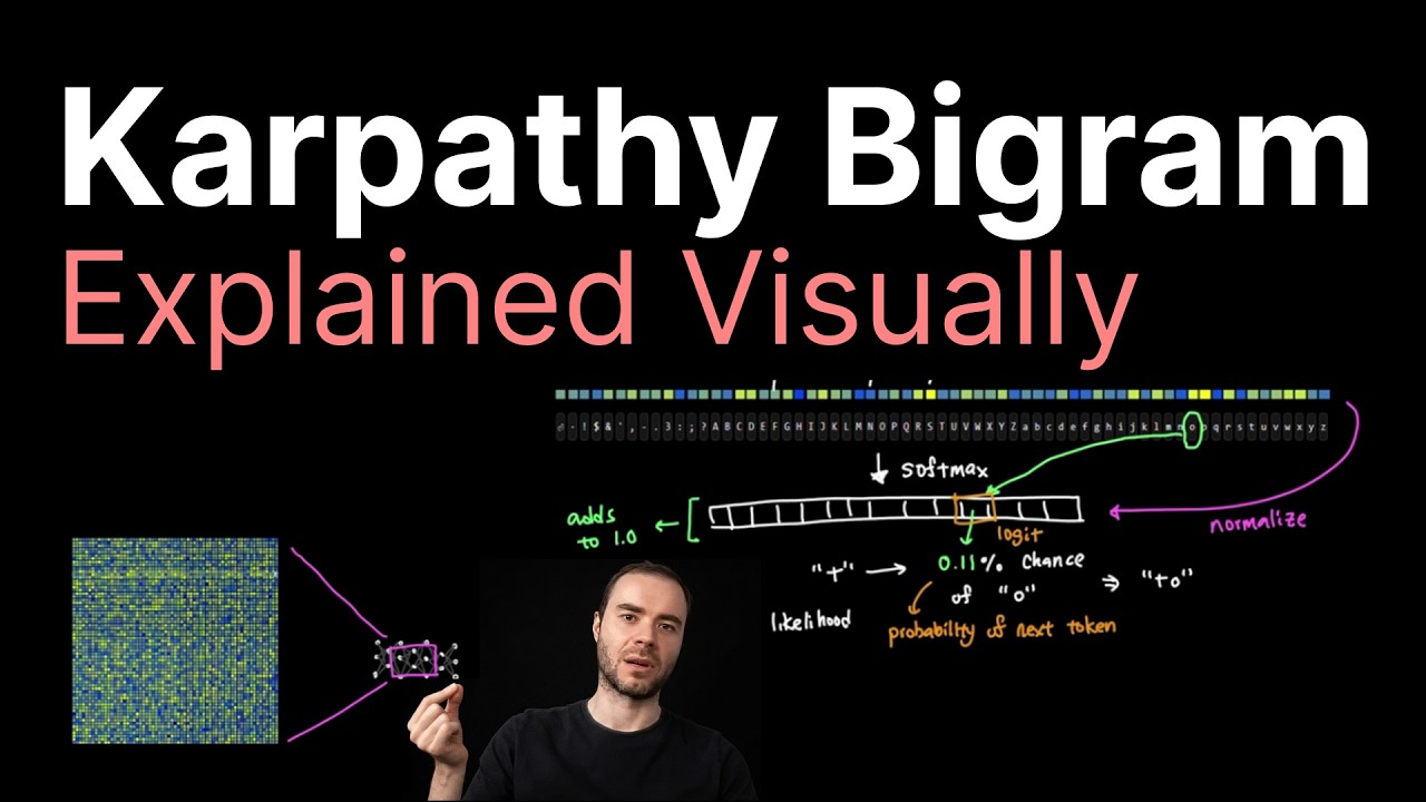And the idea is to find out just how far the model's predicted probability for the correct next token is from where it really needs to be. And this is where terms that you might have heard of before like softmax comes into play. Now, if you're wondering why we even need to think about softmax in the first place, it's because the table contains raw numbers like 0.4, 1.6, or 2.4. It's hard to know what these numbers really mean intuitively. So, what softmax does is it normalizes the row into logits that all add up to the number one. Which means if the token O says 0.11, it means that there's 11% chance that the letter O will follow after the letter T. And now given these logits that tells us the probability of the next token. What negative lo likelihood does is that it looks at the model's assigned probability for what the actual token would have been and penalizes the model when that probability is low. So, at first, our loss in the initial state that's randomly generated might read something like 4.8786. Not bad, but plenty of room to improve to drive this number down. And the goal for training is to take this average down by sampling more and more from the data set to drive our loss to the lowest asmtote to let's say a value of two or even sub two after running tens and hundreds of thousands of iterations over and over again. And there's actually a bit of art mixed with science when it comes to training. And I'm sure you've heard of people saying things like the training run is unstable. Or you hear phrases like loss is spiking during the training run. What's actually happening underneath is during training when these raw numbers are being updated to reduce the loss rate by nudging them towards the right direction a little bit at a time. There's a bit of finance in deciding how aggressively to change these numbers towards the right direction. Too big. you start to get very unstable updates and too small. It takes too long and doesn't find the lowest loss. That's why we need to run thousands and thousands of iterations and the loss will slowly go down from values like 4.7 to mid twos. And the mechanics that actually are responsible for these are back propagation that finds the gradient and the optimizer that helps stabilize these updates. So after 10,000 iterations, let's say, and bringing the loss down closer to two, this is the output that the model finally generates, which in comparison looks a lot better than what we first produced earlier given a randomized embedding. But it still looks pretty gibberish. And the reason for this sketchy result is not really in the data or in the training run itself either. The fault is actually in the model architecture itself. What we just built here is called biogram language model. And biogram language model is only designed to look back one previous token instead of the entire context. In other words, even though earlier we split the sequence to be or not to be that is the into four batches of eight blocks. The model doesn't care what previous tokens existed. It only looks at and cares about the current character and the character after that. So it can make a sentence that looks like a sentence but cannot really form a word when we need to go beyond this basic framework and now look at incorporating something more complex like the attention mechanism and adding an attention mechanism crosses over to what's called GPT architecture which will be part two of this series covering Karpathy's video mentioned earlier. So keep an eye on that.