Enjoying this issue?
Get tomorrow's AI & engineering digest in your inbox — hand-picked, summarized, and always spam-free.
TLDR
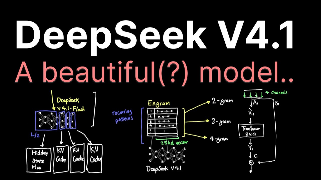
DeepSeek V4.1 Flash uses a Causal Encoder-Decoder architecture that halves prefill compute by processing input tokens through only half the model layers, while the Engram module adds 196 billion parameters dedicated to storing recurring local patterns. The model achieves a 437x reduction in per-token KV cache since 2022, but token efficiency remains a weakness.
Key points
DeepSeek V4.1 Flash introduces a Causal Encoder-Decoder (CED) architecture that uses only half the layers during prefill, cutting prefill compute in half.
The Engram module stores recurring local patterns in a separate lookup table with 196 billion parameters across two layers.
Per-token KV cache has been reduced from 389 KB to 890 bytes over three years, a 437x improvement.
Single pass MHC fuses three kernel operations into one, reducing memory transfers between GPU HBM and registers.
CSA 2 allows selective reuse of KV cache across layers through full, index, and reuse modes to further reduce memory.
Tools mentioned
Techniques
- Causal Encoder-Decoder (CED)
- Engram memory module
- Cross-layer Sparse Attention (CSA 2)
- Hierarchical sparse indexer
- Single pass Multi-Head Coefficient (MHC)
- Hash-based embedding lookup
Stop scrolling. Start reading smarter.
Receive the day's most important AI & engineering updates in one concise email. No spam.
Transcript (captions)
In just a month and a half, DeepSync publicly released the new flash model, Deepseek V4.1 Flash. And despite being just a 0.1 jump, these two are practically two different models. Now,
there's a lot of interesting ideas to go through. So, let's get right into it. What if instead of relying entirely on the model's internal parameters, we created a separate storage for recurring
patterns in language. That way, during inference, the backbone can just look them up as needed. Deepseek v4.1 flash added this module called engram. And the idea is simple in theory. We know that
given a neural network that processes input through various layers, the token representation gets contextualized and the attention mechanism pulls relevant information. And the idea is to
essentially create a separate channel where the model can still learn but isolate the memorization of recurring local patterns away from the main language backbone. Now, before we get
into the actual mechanism, it's important to keep in mind that just because we just created this alternate stream where the model can learn and hope that short-term patterns are
learned in this engram module, it doesn't mean that the main backbone won't learn them either or that learning will only happen in the engram module. Unlike traditional software engineering
where we programmatically write how different components interact with each other, in neural networks, we're creating these channels where information could flow from one place to
another. But the actual learning is determined by how gradient descent actually updates these parameters across those pathways which would then determine how these components would
actually be specialized in the end. So when we say phrases like well the purpose of engram module here is to memorize recurring local patterns while that's probably true we're really
describing the inductive bias of the architecture and it's not like coding where we describe a hard rule about where this knowledge actually needs to live and you might be wondering this
wait if what you're saying is true if I can't control how the model actually learns why are you then saying that this engram module is for memorizing local patterns how Can you say that while not
explicitly programming it that way? Deep sea created three different mechanisms for each token that gets processed. 2 g, 3 g, and 4 g. Take the current token and look back two, three, and four tokens
back to use them as an ID and create a bucket that contains 256 dimension vector. This way, if the model ever encounters the same recurring pattern, it can just look at the parameters that
are contained in this storage. Now, as much as this might make complete sense, there's one small problem with this. The number of possible IDs that we need to create for these engrams is too large.
I'm sure you remember back in your stats class in high school, you remember the idea behind permutations where say the number of permutations that a 9-digit keypad that can generate a four-digit
code is 9 to the^ of 4. So, 6561. And it's the same idea here, except in this case, it's not a nine-digit keypad, but we have to think about the entire dictionary of tokens that's used by
DeepSeek. And for this model, they use 129,280 tokens. So you can imagine what a for this case might look like. It's a big number. Which means the storage that
contains 256 dimension vectors to hold every single possible for alone will need 1.8 8 trillion H100s just to hold all possible for Grams. So clearly we need a better method. DeepSync basically
inverted this entire operation by taking this blowing up of ID from engrams into 384 million rows as the maximum. And now that we know the maximum number of keys that we have in the storage, we just
have to figure out how to make the middle layer work. What DeepSync did to make this happen is they first reduced the vocap size for the engram from 129,280
to 99,92 by consolidating a lot of similar tokens into a smaller subset. But 99,000 is still a huge number to deal with. And for each engram, DeepSync assigned eight different hash heads and
gave each of them 60 million possible rows. So given the three engrams with eight hash heads and each having 60 million rows, that puts us exactly at 384 million rows total as a maximum
number of rows regardless of how many permutations the 99,92 tokens can be arranged. Pretty cool, right? But the devil's in the math which uses a large number multiplier and bitwise exor using
large prime numbers to make all of this happen. And all of this is beyond the scope of the video, but I outlined them in my substack if you're curious. Now I mentioned earlier about the recurring
pattern and that's really the key here. What this engram table allows is a 256 dimension vectors that lives in the table that acts as a literal models parameter where given the occurrence of
these two tokens or these three tokens or these four tokens. It should give the model the ability to actually use the eight hash heads each containing 256 dimensions for learning to actually
occur in these parameters directly. And that's really the key here. These dimensions are literally the model's parameters that actually contain what the model learns during training and
also what the model can use during inference. That's why when we read through the model's notes, it lists the engram memory as 196 billion additional parameters to take account during
inference. And the math checks out here as well with the 384 million maximum rows each containing 256 dimensions embedding gives us 98.3 billion parameters. And when we look at the
models diagram, the engram portion we just saw gets injected on layer 1 and layer 15. So the engram module is actually two, which is how we get to 196 billion in total parameters. And that's
exactly what the blog post is referring to right here. So now that we created the engram module for small local memory but separated from the main backbone, the core idea is for the model to now
learn useful representation of short recurring patterns inside of those engrams in the memory slots that they have during training. Now when we bring back up the model architecture diagram,
what you probably have noticed here is this weird concept encoder and decoder. What's that all about? This is what DeepC calls causal encoder decoder or CD. then you really ought to see these
next. Ever since GPT model became the industry standard that branched off of transformer model that was first introduced in 2017. GPT essentially broke off the encoder part of
transformers and only use a decoder only. And most LMS still follow the decoder only as the industry standard. And now DeepSick's new CED is sort of bringing us back to this moment by
adding what they call causal encoder on one side of the model architecture and decoder on the other side. And you might be wondering why DeepSync would even do this. And the reason why has largely to
do with two main reasons, compute efficiency and KV cache reduction. I'm sure you've seen this diagram here with the release of the model that shows you DeepS's progression of their global KV
cache where in just past 3 years alone, Deepseek shrunk their per token KV cache from 389 kilobytes to 890 bytes, which is nearly a 437 time reduction. And the CD architecture is one of the main
reasons how Deepseek was able to further reduce their KV cache footprint by nearly four times from even their previous model only 5 months ago. So, what's really going on here? I need more
context to understand just like my agent. And that's why Firecrawl can be a great option who's sponsoring this video. If there's one thing your agent needs, it's context. And not just any
context, but context that lives on the internet. Here, I'm connecting my coding agent with Firecross MCP. And since I often use AI to help me research using SLS search, you can pull together over
43 million research papers that's indexed on highly credible scientific papers, which means I can now ask my agent to research about the emerging attention mechanism in AI to get updated
information right away. Even for developers, this could be huge given that they have indexed over 70 million developer documents. This is really important because models are often
shipped with knowledge cutoff, meaning the rest is up to the agent to actually gather up-to-date and relevant information. Firecrawl searchs can take my prompt about latest technique in post
training and because they've indexed a large body of documents already, it can help narrow down where to look and only return relevant excerpts related to my prompt, which also helps save cost
consistently by 90% across many benchmarks. You can try Firecrawl for free without an API key. Link in the description below. Ever since context windows started being 1 million in size,
which became sort of like a standard that everyone expects now, this large context window put a huge strain on the amount of compute that it takes and also the amount of KV cache that it needs to
actually hold in the memory somehow. For reference, going back to the original transformer model that was first introduced back in 2017, if we just took this vanilla transformer architecture
and used the same model architecture as Deep Sigv 4.1 flash, a 1 million context window would need a KV cache around 819 GB. Huge, right? And the complexity is roughly around O of L * N * D where L is
the number of layers, N is the length of the sequence which is 1 million and D is a hidden dimension which in Deep's case is 5,120. And over the years since 2017, we had a
lot of different attempts being made by a lot of different labs trying their own unique way of bringing this number down to something more manageable. Because 819 GB for a single user will need
around at least 11 H100. And that's unacceptable. And some notable attempts includes like reducing the size of KV entry itself or maybe quantizing the KV cache itself, limiting the attention by
using sliding window attention or sparse attention, reeving KV cache across layers, evicting KV cache or even deepseek's previous approach in V4 model that introduced CSA and DSA on top of
lightning indexer. And you might have heard of some or all of these above. And all of these are valiant efforts to try to manage this growing complexity with the KV cache. So what if given the 1
million context, instead of using the entire models layers, we only use half of the layer during prefill. When I pull up Open Router and see how Deep Seek V4.1 is actually being used in
production, a large majority of these models usage is actually dominated by prompt, which is the input tokens that's being processed rather than output tokens or reasoning tokens that's being
generated by the model. So targeting this exact blue line here and only using half of the model during that would mean a lot of efficiency being added right off the bat, right? But how exactly does
this work where you only use half of the model's layer when it processes input tokens from prefill? The idea actually dates back a few year called Yoko or you only cache once and the paper introduced
this concept called decoder decoder LLM as you can see and on paper it was pretty promising. So let's say the model has 40 layers in total. It would only build KV cache on the first half of the
model. And instead of traditional transformer that would build KV cache for each layer, it would build a global KV cache which means now every layer subsequent to layer 20 which is
referenced the same builtup global KV cache which dramatically reduces the KV cache footprint. That was the idea behind Yoko and DeepS saw this and built on this idea. But they thought that
accessing the same global cache for subsequent layers didn't really allow the model to be expressive and the trade-off wasn't really all that worth it. So Deepseek CED keeps the layer 20's
hidden state as a common source but also allows the subsequent layers to have their own layer specific KV states allowing the layers to have their own learned projection. And I want to bring
back what I said earlier in the video, which is unlike traditional programming, we're not exactly telling the model at this specific layer, we can say, well, you should store grammar and you should
store syntax here and so on. We're actually just allowing more room for information to communicate and letting the gradient descent determine how these projections will specialize based on how
it best helps to reduce the loss. So mathematically it would be represented something like this where the hidden state for the L divided by two which for a 40 layer model would be the 20th
layer. And now the KV cache for the current layers learned KV projection is then multiplied on top. And the Z part here has more to do with CSA which we'll soon get into. So during prefill where
input tokens are being processed, the model would now only use half of the model to build and build the shared hidden representation. And during decode, every token will now run through
entire 40 layers of the model. That's why the model is 8 billion active for prefill and 16 billion active for decode, which is double the activation because the split between the prefill
and the decode part determines the depth of the layer that's actually being used. In other words, the big win here when it comes to CED is the prefill compute, which is now nearly cut in half. And
that's still a big win because we just saw how dominant prefill part is in relation to decode part in production environments. Okay, but we do have to take one more step backwards before we
actually move forward. When we moved away from Yoko to now CED, we did have to compromise on one aspect since clearly Yoko takes up the least amount of KB footprint since all subsequent
layers can reuse the exact same global KV memory instead of each storing their own layer specific version. And DeepSync didn't really want to lose out too much on the inefficiency they just added back
on by letting CD have the second half of the model store their own KV cache. And DeepSick's answer to this problem was using CSA 2. The concept behind CSA isn't really anything new by the way.
It's something that we was already introduced in their previous model, DeepSync V4 with ACA and CSA, which is something that I already covered extensively in my previous video. But
CSA 2 is an optimization built on top of CSA. So that allows some efficiency gain between these layers by introducing these three different modes, full mode, index mode, and reuse mode. I know a lot
to keep track of, but I promise it's actually easier than it looks. What you have to keep in mind here is this. The entire reason why we're even talking about this CSA is to try to reduce the
burden of having each layer having its own learned KV. So CSA 2 is really the inner mechanism that allows you to reuse parts of the global KV state across many layers instead of forcing every layer to
independently build their own KV. So full mode essentially acts as a reset where the layers build their own fresh KV states for itself and indexes them to produce top K which then gets added to
the core attention. And reindex, as the name suggests, reuses the previous global KV from the previous full layer, but generates a new query for the current layer and runs the indexer again
to choose the new top K, which adds a bit of a compute overhead, but certainly not as big as rebuilding the complete new KV state for that layer. And finally, the reuse mode is even cheaper
where it keeps both the global KV in the same top case selection and lets the current layer simply compute its own attention over those previously selected KV entries without rebuilding or
reindexing anything. So these are essentially tools that CSA 2 now comes with. And when you look at the model architecture diagram here, it shows you just how it embeds different modes
across different positions of the layers as you can see, which directly means that the compromise that we reintroduced layer KV with the CED is now optimized without having to have each layer forced
to have its own KV. But we can be a little bit more selective about how both the encoder and decoder works through the KV along the way. One interesting thing that you might have noticed here
is that the CSA ratio is either one or two here. But back when CSA was originally introduced in V4, they defaulted to 4:1 ratio. Another thing that you might have noticed here is this
arrow called hierarchical sparse indexer. This is illustrated here where DeepC grouped the positions into blocks of eight and finds the biggest score in that block and keeps the top 48 blocks
as candidates. which means there's now a total of 16,384 positions that the reindex can now search from instead of looking through the entire global context again. Now,
there's one more thing that we need to pick out here, which is this thing, single pass MHC. If you remember my previous video talking about when MHC was first introduced by Deepseek, it's
one of those optimizations that DeepSseek made in the residual network where instead of just adding the input back to itself after the transformer block, MHC separates them into four
channels to allow the model to be more selective and also more expressive over how the inputs are actually passed down. But what in the world is a single pass MHC? To understand why single pass MHC
is important, we need to dig into the hierarchy of memory in the GPU. And this is literally my favorite topic to talk about which is how data moves and gets processed in the graphics cards. We know
that largely GPU has HBM which is the most abundant storage that stores things. And when we get into the SM modules, we have other things like L2, L1 cache and registers that are actually
meant to hold temporarily or run computation on. And unlike HPM, memory here is very very low. Like going from 80 GB in H100 to like 50 megabytes in L2 cache that's shared chipwide. And each
SM module has about 256 kilobytes of register files. And because of this disparity in memory that's available, what typically ends up happening is that whenever there's a complicated algebra,
especially ones where the output of one portion of the algebra depends on another, data needs to be constantly written and read back and forth from the register to HPM and from HPM back to the
register. And each time data unnecessarily travels between these two means inefficiency, especially at scale. And the original MHC is just one of those things that has this kind of
algebra where dependencies force data to travel back and forth just to make one single forward pass to happen. Now you might look at this and say, "Wow, why even bother changing the original
residual network into something like this where you got this complex plumbing for information to travel?" And the answer to that is really going back to how I said earlier that unlike
traditional coding where we can just add and change the code to get specific behavior out of the model, things are different in neuronet networks where we have to create these additional plumbing
for more pathways where information can flow. Which means gradients can now specialize each inlet we added to do something more special. And in the case of MHC, it's all about giving the model
a chance to decide how much information should move through the blocks. So if we add the mathematical notation here, it means we're now giving the model to actually start learning these
coefficients A, B, and C that determine how information is mixed and carried forward. But the problem with the original MHC was that the read and write in the kernel was very inefficient. More
formally written, this mathematical operation actually breaks down into three kernel operations like this where the first kernel tries to find the value of the A, B and C coefficients. Second
kernel operation uses the A to apply the current input X to find the X hat. And the last operation is the actual computation to find the output using all the variables that we now have. Now
because of these three kernels, the actual transportation between HPM and SM in the physical world looks something like this where you have to have many reads and some writes happening back and
forth. If we counted each residual, we now have 13D reads and 4D writes and after factoring porm we have in total 20d operations happening. were formerly written this inefficiency can be
represented as 4n + 4d which by putting n= 4 in our case also puts us at 20d operation and the lower bound here that we should aim for is 2 n + 2d and that's exactly what a single path MHC tries to
achieve here by removing these three kernels and making them into one. Now you might think that this is a fused kernel operation but that's actually later on which is the mega MHC but
single pass MHC isn't cramming these into one kernel but changing the algebra that we saw earlier so that the temporal dependency in the order of operations is shifted so that the variables that needs
to be known at runtime is available then and there now. And the trick was to change the a coefficient to shift one block backwards and using them instead. This way single kernel operation can
actually pull all the required variables and run them at once. That is the optimization that single pass MHC here achieved. Now looking at the diagram now we see that in this video we covered
engram that acts as a recurring local patterns to be stored and fed into layer 1 and layer 15. Here we also walk through CED architecture that separates the prefill and the decode to save
compute during prefill and the CSA 2 mechanism that can selectively add additional efficiency in reusing previous layers main KV or indexer or both an additional KV compression that
CSA does on top. We also went through hierarchical sparse indexer that allows candidates of 248 blocks to reuse and finally a single pass MHC that adds kernel optimization on how memory flows
between HPM to the register in residual network. All in all this is really a beautifully crafted model from deepseek and I really enjoyed reading this paper learning about all the inner mechanics.
I do think though that when it comes to how the model actually performs in production, Deepc could really start improving the token efficiency, which currently scores one of the worst out
there. But given that the model has huge cost efficiency and memory efficiency and how fast the model now runs at over 100 tokens per second, I think these currently act as a buffer for people to
choose this model. But cost efficiency is not really a strong leg to stand on. But the token efficiency and intelligence is what I hope Deep Seek to continue pushing forward just like they
did when they released their R1 model. Now, if you want more detailed breakdown of how I did my research for this model, you can read them on my Substack. I'll have the link available below.